The Silent Degradation Problem: Why AI Demand Models Drift Undetected
Most AI demand planning failures do not announce themselves. Forecasts continue flowing into your planning system, dashboards remain green, and S&OP meetings proceed without alarm. Meanwhile, the model has quietly stopped being right — its learned relationships between features and demand no longer reflect the world it is operating in.
This is model drift, and its defining characteristic is invisibility. Unlike a system outage or a data pipeline failure, drift does not produce error messages. It produces slightly wrong forecasts that accumulate into materially wrong inventory positions over weeks and months.
The business cost is measurable. Organizations relying on manual monitoring and fixed retraining schedules — typically every three to six months — carry 12–20% excess inventory costs compared to teams using drift-triggered retraining approaches, according to research cited in the DriftGuard hierarchical drift detection framework (referencing CSCMP 2023 State of Logistics data). In controlled experiments on over 30,000 time series from the M5 retail dataset, WMAPE degraded from 0.048 to 0.192 as drift went undetected — a fourfold accuracy collapse that would be catastrophic in any production planning environment.
The five-stage framework in this guide — drift taxonomy, monitoring architecture, ensemble detection, SHAP-based diagnosis, and tiered response with retraining governance — is designed to treat drift management as a continuous operational discipline rather than an occasional maintenance event.

Drift Taxonomy for Demand Planning: Three Failure Modes and How They Propagate
Not all drift is the same, and treating it as a single phenomenon is one of the most common sources of misdiagnosis in production demand planning environments. Conflating data drift with concept drift leads to applying the wrong remediation — wasting compute on full model rebuilds when a targeted feature correction would suffice, or vice versa.
Three distinct failure modes are relevant to demand planning AI systems, as defined by IBM's model drift taxonomy and operationalized in the DriftGuard research:
| Drift Type | What Changes | Relationship to Demand | Detection Signature | Primary Remediation |
|---|---|---|---|---|
| Concept Drift | The relationship between input features and demand changes | Feature-to-demand mapping is no longer valid | WMAPE degradation without input distribution change | Model retraining or architecture review |
| Data / Covariate Drift | The distribution of input features shifts | Feature-to-demand relationship may still be stable | PSI or KS-test flags on input features before error rises | Feature pipeline correction or retraining on recent data |
| Upstream Data Change | Pipeline-level changes — unit-of-measure switches, currency conversions, data schema changes | No real-world demand shift; labeling changes create artificial signal | Sudden step-change in a single feature distribution; error spikes without demand event | Pipeline correction; retrain only after data is normalized |
Regression-based demand forecasting models — which use external features like promotions, pricing, weather, and macroeconomic indicators alongside historical sales — are more vulnerable to concept drift than pure time-series models. Higher feature dimensionality means more relationships that can break. A competitor entering a market, a promotional strategy shift, or a regional economic contraction can invalidate learned feature weights without changing the input data distribution in ways that simple error monitoring will catch quickly.
Hierarchical Propagation: Why SKU-Level Drift Creates Enterprise-Level Surprises
Demand planning models operate across a hierarchy: individual SKUs roll up to categories, categories to regions, regions to enterprise totals. Drift at the SKU level does not propagate cleanly through this hierarchy — it amplifies in some paths and cancels in others, depending on the direction of individual forecast errors.
A category with half its SKUs over-forecasting and half under-forecasting may show acceptable aggregate WMAPE while individual SKU service levels are collapsing. Conversely, a cluster of SKUs all drifting in the same direction — a common outcome when a shared feature like a promotional calendar changes — can produce regional-level bias that looks catastrophic in aggregate even when individual SKU errors appear modest.
Monitoring Architecture: KPIs, Thresholds, and S&OP Cycle Alignment
A monitoring architecture for demand planning drift needs to track two distinct signal types: error-based metrics that measure model output quality, and feature distribution metrics that measure input data health. Relying exclusively on error-based monitoring means catching drift late — typically after 12 days of degradation — because forecast errors must accumulate to statistical significance before they exceed normal variance bands.
Feature distribution monitoring catches distributional shifts before they fully propagate into forecast errors, providing the early warning window that error-based monitoring cannot.
| KPI | What It Measures | Detection Signal Type | Recommended Threshold | S&OP Cadence |
|---|---|---|---|---|
| WMAPE Degradation Rate | Week-over-week change in weighted mean absolute percentage error | Error-based (lagging) | >15% relative increase over rolling 4-week baseline | Review at weekly S&OP pre-meeting |
| MAE Bias Trend | Directional bias in mean absolute error — systematic over- or under-forecasting | Error-based (lagging) | Sustained positive or negative bias >10% of mean demand for 3+ weeks | Review at monthly S&OP cycle |
| Population Stability Index (PSI) | Distribution shift in categorical input features (e.g., promotion type, product tier) | Feature distribution (leading) | PSI > 0.2 indicates significant shift; > 0.25 triggers alert | Run weekly; flag before S&OP lock |
| Kolmogorov-Smirnov Test | Distribution shift in continuous input features (e.g., price, inventory level, weather index) | Feature distribution (leading) | p-value < 0.05 with Bonferroni correction for multiple features | Run weekly on feature snapshot |
| CUSUM Cumulative Deviation | Cumulative sum of deviations from expected error — detects gradual drift that stays below single-period thresholds | Error-based (leading for gradual drift) | CUSUM statistic exceeds 5× baseline standard deviation | Monitor continuously; alert on breach |
Aligning monitoring cadence to S&OP rhythms rather than arbitrary calendar schedules matters for operational integration. A weekly feature distribution scan timed to run before the statistical forecast lock gives planners actionable information at the point they can act on it — not days after the consensus number has been published.
Ensemble Detection: Why Single-Method Monitoring Fails and How to Fix It
Each individual drift detection method has a structural blind spot that makes it unreliable as a standalone signal:
- Error-based RMSE comparison is slow — it requires 12+ days of accumulated forecast errors to confidently distinguish drift from normal demand variance, by which point significant damage to inventory positions may already be underway.
- Statistical tests (KS, PSI) detect input distribution shifts but are blind to concept drift — a model can fail on unchanged input distributions if the learned relationship between features and demand has become invalid.
- Autoencoder anomaly detection identifies unusual patterns in input data but is sensitive to normal seasonal variation, generating false positives during predictable demand cycles if not carefully calibrated.
- CUSUM change-point analysis excels at detecting gradual drift that stays below single-period thresholds but is slow to confirm sudden step-change events and requires careful baseline window selection.
The solution is an ensemble approach that combines all four methods and uses majority voting to produce a single high-confidence signal. The DriftGuard framework implements exactly this architecture — requiring agreement from at least three of the four detectors before triggering a drift alert. This majority-voting mechanism suppresses false positives from any single method while preserving the early detection advantage of feature distribution monitoring.

The performance case for ensemble detection is grounded in the DriftGuard research, evaluated on over 30,000 time series from the M5 retail dataset. The ensemble approach achieved 97.8% detection recall within 4.2 days — compared to a 12-day latency for error-based monitoring alone. The false positive rate was approximately 3.2%, translating to roughly one unnecessary retraining trigger per month in a typical deployment.
A false positive rate of 3.2% is operationally acceptable because the cost of one unnecessary automated retraining run is low relative to the cost of missing a genuine drift event. This asymmetry — cheap false positives, expensive false negatives — should guide threshold calibration decisions throughout your monitoring architecture.
SHAP-Based Root-Cause Diagnosis: Finding What Drove the Drift
Detection tells you that drift has occurred. Diagnosis tells you why — and which response to apply. Skipping diagnosis and defaulting directly to full model retraining is the most common and most expensive mistake teams make after a drift alert fires.
SHAP (SHapley Additive exPlanations) feature attribution provides the diagnostic mechanism. By comparing each feature's contribution to forecast errors during a stable baseline period against its contribution during the drift period — the delta between these attribution vectors — you can identify precisely which features are driving the increased error. A promotional calendar feature that contributed minimally to baseline error but now accounts for 40% of drift-period error is a clear diagnosis: the promotion encoding has changed or the model's learned response to promotions is no longer valid.
This analysis aggregates across the SKU-to-store-to-region hierarchy to produce a diagnostic map showing drift severity at each level. The map answers three questions that determine the appropriate response:
- Which features are the primary drivers of increased error? (Determines whether retraining, feature correction, or pipeline investigation is needed.)
- At which hierarchy level is drift most concentrated? (Determines whether the response should target individual SKUs, a product category, a region, or the global model.)
- Is the drift pattern consistent across affected SKUs, or idiosyncratic? (Consistent patterns suggest a shared feature problem; idiosyncratic patterns suggest SKU-specific data issues.)
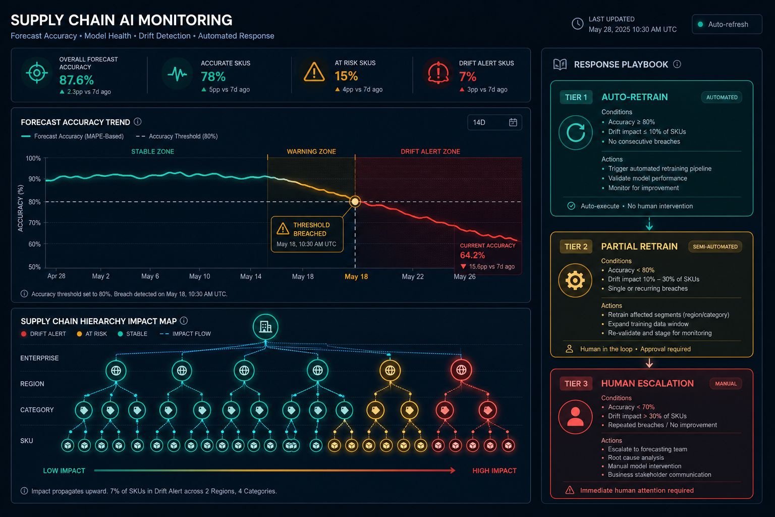
Tiered Response Playbook: Matching the Intervention to the Drift Severity
Not every drift event warrants the same response. A tiered playbook keyed to drift severity — informed by the SHAP diagnostic output — prevents both over-response (expensive full rebuilds for minor distributional shifts) and under-response (automated retraining for severe drift that requires human judgment).
| Tier | Drift Severity | Distributional Shift | Trigger Condition | Response Action | Human Involvement |
|---|---|---|---|---|---|
| Tier 1 — Mild | Low | 10–15% shift in input distributions | 3-of-4 ensemble vote with SHAP delta below moderate threshold | Automated retraining with optimized training window selection; deploy after validation gate passes | None required; automated alert to planning team after deployment |
| Tier 2 — Moderate | Medium | 15–30% shift; SHAP identifies concentrated feature drivers | 3-of-4 ensemble vote with SHAP delta indicating top-K SKU concentration | Targeted partial retraining of the 15–20% most severely affected SKUs; other models unchanged | Data science team reviews SHAP diagnostic before retraining; planner notified of affected SKUs |
| Tier 3 — Severe | >30% distributional shift; accuracy recovery incomplete after retraining | Ensemble vote unanimous; SHAP shows broad feature attribution collapse | Automatic remediation insufficient; human escalation triggered | Planner escalation; potential model architecture review; manual override of affected forecasts during investigation | Required — supply chain planner and data science lead must jointly assess before any model change |
Tier 3 events — severe drift exceeding 30% distributional shift — represent situations where the model's learned structure may be fundamentally misaligned with current market dynamics. Examples include a major competitor entering a product category, a sustained economic contraction changing consumer purchasing patterns, or a structural shift in a promotional strategy that invalidates years of learned promotional response curves. In these cases, automated retraining on recent data may produce a model that is better than the drifted version but still structurally inadequate. Human review of model architecture is warranted.
Retraining Governance: Event-Driven Triggers, Window Selection, and Validation Gates
Fixed-schedule retraining — running every 30, 60, or 90 days regardless of whether drift has occurred — is the dominant practice in most organizations. It has two structural problems: it wastes compute during stable periods when retraining provides no accuracy benefit, and it responds too slowly during periods of rapid drift when the next scheduled retrain may be weeks away.
Event-driven, threshold-based retraining triggers solve both problems. Retraining fires when the ensemble detection layer confirms drift, not on a calendar. During stable periods, no unnecessary retraining occurs. During drift events, the response begins within days of detection rather than waiting for the next scheduled window.
Training Window Selection by Drift Type
The training window used for retraining should be selected based on the drift type identified in the diagnostic phase, not applied uniformly:
- Sudden drift (step-change events such as a market entry or a supply disruption): use a short training window of approximately 30 days, excluding pre-drift data. Including pre-drift data trains the model on a world that no longer exists.
- Gradual drift (slow structural shifts such as changing consumer preferences or incremental pricing strategy changes): use a longer window of 90–180 days. Short windows will underfit on gradual drift because recent data alone does not contain enough signal to distinguish the new pattern from noise.
- Upstream data change (pipeline-level schema or unit changes): correct the data pipeline first. Retraining before the pipeline is normalized will encode the corrupted data into the new model.
The ROI Validation Gate
Before deploying a retrained model to production, a validation gate should estimate whether the expected accuracy improvement justifies the retraining compute cost. This is not a high-friction approval process — it is a lightweight automated check that prevents unnecessary retraining from being deployed when the accuracy delta is within normal variance.
The economic case for selective retraining over full-portfolio retraining is substantial. DriftGuard's research demonstrated up to 417× ROI by retraining only the 15–20% most affected models in a portfolio of 30,000+ time series rather than retraining all models uniformly. The majority of models in a large portfolio are not drifting at any given time — retraining them wastes compute without improving accuracy.
Human Approval Gates in the Retraining Pipeline
The AWS SageMaker Model Monitor architecture illustrates a practical two-stage governance model: a data scientist approves the retrained model for staging after reviewing training metrics, and an operations team approves promotion to production. This cross-functional gate structure prevents automated retraining from bypassing human judgment for high-stakes model changes — particularly relevant for Tier 2 and Tier 3 drift events.
Tooling Landscape: Selecting a Drift Monitoring Platform for Supply Chain Contexts
The model monitoring tool market includes several platforms with meaningful capability differences for supply chain contexts. The evaluation criteria that matter most in demand planning environments differ from generic MLOps monitoring requirements.
| Tool | Multi-Model / Hierarchical Series Support | Native Supply Chain Metrics (WMAPE, MAE Bias) | Explainability Overlays | Enterprise Scalability | Audit Trail | MLOps Pipeline Integration |
|---|---|---|---|---|---|---|
| Evidently AI | Yes — supports batch and streaming monitoring across model portfolios | Configurable; requires custom metric definition for WMAPE | Feature drift reports with SHAP integration available | Open source core; enterprise tier for scale | Report-based; exportable | Python-native; integrates with MLflow, Airflow |
| Arize AI | Strong multi-model support; hierarchy requires custom configuration | Configurable custom metrics; no native WMAPE out of box | SHAP-based feature importance monitoring built in | Designed for enterprise scale | Full audit log with time-stamped events | Native integrations with major MLOps platforms |
| NannyML | Batch monitoring; less suited to real-time streaming | Configurable; strong on performance estimation without ground truth | SHAP integration available | Mid-market to enterprise | Limited native audit trail | Python library; integrates with standard pipelines |
| AWS SageMaker Model Monitor | Strong for AWS-native deployments; multi-model via Model Registry | Configurable; requires custom metric definition | Limited native explainability; integrates with Clarify for SHAP | Enterprise scale within AWS ecosystem | CloudWatch logs; EventBridge event trail | Native EventBridge-to-pipeline automation; strongest detect-alert-retrain loop |
| MLflow | Model registry supports multi-model tracking; monitoring requires plugins | No native drift monitoring; requires custom implementation | No native explainability overlay | Open source; enterprise via Databricks | Experiment tracking; not purpose-built for operational audit | Strong integration with Spark, Databricks pipelines |
| WhyLabs | Multi-model support; profiling-based approach | Configurable custom metrics | Feature importance drift tracking available | Enterprise scale | Profile-based audit history | REST API; integrates with major ML frameworks |
For organizations operating on AWS infrastructure, the SageMaker Model Monitor architecture provides the tightest detect-alert-retrain automation loop: CloudWatch metrics breach a threshold, EventBridge fires a rule, and a SageMaker Pipeline retraining job starts automatically. For organizations on a multi-cloud or platform-agnostic stack, Evidently AI or Arize AI provide more deployment flexibility with comparable drift detection capability.
Implementation Roadmap: Four Phases, Success KPIs, and Common Failure Modes
Operationalizing drift management is a phased effort. Attempting to deploy the full ensemble detection and SHAP diagnosis stack in a single initiative typically fails because the organizational prerequisites — baseline KPI definitions, ground-truth pipelines, planner escalation protocols — are not in place to support it. The four-phase roadmap below sequences the work in order of dependency.
- Phase 1 — Baseline Instrumentation: Define your monitoring KPI set (WMAPE, MAE bias, PSI, KS-test, CUSUM). Establish baseline distributions for each metric using 90 days of historical production data. Set initial detection thresholds — start conservative (higher false positive tolerance) and tighten after observing false positive frequency in production. Verify that your ground-truth label refresh pipeline is operational and current.
- Phase 2 — Ensemble Detection Deployment: Deploy the four-method ensemble detection layer. Run in shadow mode for 4–6 weeks alongside your existing monitoring approach to calibrate majority-voting thresholds and validate detection latency against known drift events in your historical data. Align alert cadence to S&OP cycle touchpoints.
- Phase 3 — SHAP Diagnosis Integration and Response Playbook Operationalization: Integrate SHAP attribution comparison into the drift alert workflow. Build the hierarchical diagnostic map aggregating from SKU to region. Define the Tier 1 / Tier 2 / Tier 3 classification criteria for your specific model portfolio and business context. Conduct tabletop exercises with planning and data science teams to validate escalation protocols before a live Tier 3 event occurs.
- Phase 4 — Retraining Governance Formalization and ROI Tracking: Replace fixed-schedule retraining with event-driven triggers. Implement the ROI validation gate before production deployment. Establish a retraining log that captures drift type, severity tier, training window selected, validation gate outcome, and post-deployment accuracy delta. Review the log monthly to identify systematic patterns and refine threshold calibration.
Success KPIs
Track these metrics to evaluate whether your drift management framework is performing as intended:
| KPI | Definition | Target Direction |
|---|---|---|
| Drift Detection Latency | Days from drift onset to confirmed ensemble alert | Reduce toward 4–5 day target |
| False Positive Rate | Proportion of alerts that do not result in confirmed drift after SHAP diagnosis | Maintain below 5%; investigate spikes |
| Retrain-to-Recovery Time | Days from retraining trigger to production WMAPE returning to baseline | Reduce; benchmark against pre-framework baseline |
| Selective Retraining Rate | Proportion of retraining events that are Tier 1 or Tier 2 (targeted) vs. full-portfolio | Increase toward 80%+ selective |
| Inventory Cost Delta | Change in excess inventory carrying cost attributable to improved forecast accuracy post-framework deployment | Reduce; requires finance partnership to attribute |
Common Failure Modes
Organizations that have attempted drift management frameworks report consistent failure patterns. Knowing them in advance prevents repeating them:
- Monitoring without diagnosis. Teams deploy ensemble detection but skip SHAP integration. Every alert triggers a full model rebuild because there is no principled basis for selective retraining. Compute costs escalate, and planning teams lose confidence in the framework.
- Fixed-schedule retraining persisting alongside event-driven triggers. The new event-driven system is deployed but the old monthly retrain job is not decommissioned. Models are retrained on conflicting schedules, making it impossible to attribute accuracy changes to drift events or to calibrate the ROI validation gate.
- Missing ground-truth label refresh. Event-driven retraining fires correctly, but the training data has not been updated with recent actuals. The retrained model is trained on the same stale data as its predecessor and reproduces the same drift within weeks.
- No planner escalation protocol for Tier 3 events. Severe drift events trigger alerts that no one has been designated to act on. The framework correctly identifies a crisis but the organizational response path does not exist. Build the escalation protocol in Phase 3, not after the first Tier 3 event.
- Threshold calibration set once and never revisited. Detection thresholds set at implementation reflect the demand patterns and data quality of that moment. As your product portfolio, data pipelines, and market context evolve, thresholds need systematic recalibration — at minimum quarterly, or after any significant business change.
Comments
Join the discussion with an anonymous comment.