The Seasonal CPG Forecasting Problem: Why One Number Is Never Enough
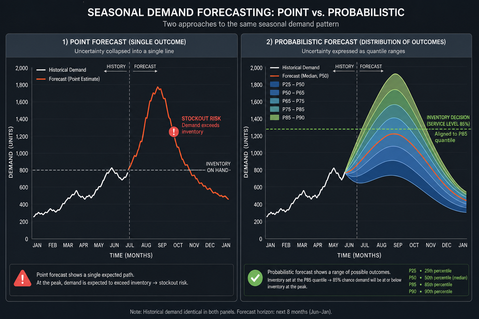
Every summer, holiday, and back-to-school cycle, CPG supply chain teams face the same structural problem: they have one forecast number per SKU per period, and reality almost never lands exactly on that number. When demand spikes 40% above the point estimate during a July promotion, the result is a stockout. When it comes in 30% below after an over-ordered seasonal push, the result is markdown losses. The single number in the planning system does not tell you how likely either outcome is — it just tells you what the model expected.
This is the core problem that separates demand forecasting methodology for seasonal CPG from demand forecasting for stable, evergreen products. Seasonal and promotional SKUs have demand distributions that are wide, asymmetric, and often fat-tailed. A single point estimate — no matter how sophisticated the model that produced it — collapses that entire distribution into one number and discards everything else. The uncertainty does not disappear; it simply becomes invisible to the planning system.
For CPG teams managing portfolios that include both stable core SKUs and high-variance seasonal or promotional items, the question is not which methodology wins universally. It is which methodology fits which part of the portfolio — and what the cost of using the wrong one looks like during a demand spike.

How Traditional Statistical Forecasting Works — and What It Was Designed For
The workhorses of demand forecasting in CPG — ARIMA, exponential smoothing, Holt-Winters, and moving averages — were designed to identify patterns in historical demand and project those patterns forward. Each method produces a single deterministic value for every future period: one number for week 12, one for week 13, and so on.
These methods have real strengths that should not be dismissed. For stable, slow-moving SKUs with consistent demand patterns and low week-to-week variance — a core grocery staple, a household cleaning product with flat year-round demand — they are computationally inexpensive, interpretable, and often accurate enough to support effective replenishment. A demand planner can inspect the model parameters, understand why the forecast moved, and explain it to a commercial team.
The issue is not that these methods are wrong in principle. It is that they were built for a problem where the central tendency of demand is the primary decision-relevant quantity. When the distribution of possible demand outcomes is narrow and roughly symmetric, knowing the expected value is sufficient. The safety stock buffer handles the residual uncertainty.
- ARIMA (AutoRegressive Integrated Moving Average): captures autocorrelation in demand history and projects forward; requires stationary or differenced series; produces a single conditional mean forecast per period.
- Exponential smoothing: weights recent observations more heavily than older ones; variants like Holt-Winters add trend and seasonal components; output is a single smoothed projection.
- Moving averages: simple average of recent periods; directionally useful for stable demand but slow to respond to structural changes or demand spikes.
- Regression-based methods: model demand as a function of explanatory variables (price, promotions, seasonality index); still output a single point estimate per period, typically the conditional mean.
All of these methods produce the same structural output: one number. That number is typically the expected value — the mean of the distribution the model implicitly assumes. What happens to the rest of the distribution is the subject of the next section.
The Point-Estimate Trap: How Collapsing Uncertainty Distorts Inventory Decisions
When a point-estimate forecast feeds into safety stock calculations, the math requires an assumption about the shape of the forecast error distribution. The textbook formula — safety stock equals the standard deviation of forecast error multiplied by a service factor derived from the normal distribution — embeds a specific assumption: that demand forecast errors are normally distributed around the point estimate.
For seasonal CPG products, this assumption is routinely violated. Demand during a promotional event or a seasonal peak is not symmetrically distributed around the forecast. It can spike dramatically on the upside when a promotion outperforms, and collapse on the downside when a weather event delays purchasing. The distribution is skewed, often right-tailed, and sometimes multimodal when multiple demand drivers interact. A Gaussian safety stock buffer calibrated to that symmetric assumption will systematically underprotect against upside demand spikes and overprotect against downside scenarios.
This observation — from Lokad, a vendor with a commercial position in the forecasting market and therefore a source to contextualize appropriately — points at a structural flaw that is widely acknowledged in supply chain practice. The reorder point formula (reorder point = lead time demand + safety stock) only works as intended when the distribution of demand over the lead time is known and correctly specified. If the distribution is non-normal and the formula assumes normality, the resulting reorder points will be systematically miscalibrated.
For a stable evergreen SKU, this miscalibration may be tolerable — the errors are small and the cost of a stockout or overstock is modest. For a seasonal SKU with a short selling window, a promotion that doubles baseline demand, or a weather-sensitive product category, the miscalibration compounds. The stockout during a peak week costs not just the lost margin on that week's sales, but potentially the entire seasonal opportunity.
What Probabilistic Demand Forecasting Actually Outputs
Rather than collapsing the future demand distribution into a single expected value, probabilistic demand forecasting outputs the shape of the distribution itself — or a set of quantiles that characterize it. A probabilistic forecast for week 12 might report: P50 demand of 1,200 units, P75 demand of 1,650 units, and P90 demand of 2,100 units. The planner can now see not just what the model expects, but how wide the range of plausible outcomes is and how much extra inventory would be needed to cover the 90th percentile scenario.
Several methodological approaches produce this type of output:
- Quantile regression forests: non-parametric ensemble models that estimate multiple quantiles of the demand distribution simultaneously without assuming a parametric distribution shape. Capable of fitting fat-tailed and asymmetric distributions.
- Deep learning with distributional heads: neural network architectures (including Mixture Density Networks) that output parameters of a probability distribution rather than a point estimate. Structurally probabilistic and able to model complex non-linear demand patterns.
- Bayesian structural time series: explicitly models uncertainty through prior distributions and posterior updates; produces full posterior predictive distributions over future demand.
- Monte Carlo simulation: generates many possible demand scenarios by sampling from distributions over demand drivers; the resulting scenario set characterizes the full distribution of possible outcomes.
- Gradient boosted ensemble methods: when trained with quantile loss objectives, these models can output multiple quantile estimates rather than a single conditional mean.
The accuracy metrics for probabilistic forecasts also differ from those used for point estimates. MAPE and MSE measure how close a single number is to the actual outcome. Probabilistic forecasts require metrics that evaluate the quality of the full distribution — primarily CRPS (Continuous Ranked Probability Score) and pinball loss, which penalize forecasts that assign low probability to outcomes that actually occurred and reward well-calibrated uncertainty estimates.
Why Seasonal CPG Dynamics Amplify the Gap Between Methods
The methodological difference between point-estimate and probabilistic forecasting matters most when demand distributions are wide, non-normal, and shaped by factors that interact in complex ways. Seasonal CPG supply chains concentrate several of these factors simultaneously.
- Promotional uplifts and cannibalization: A promotion on a seasonal beverage can double or triple baseline demand in a given week, while simultaneously suppressing demand for adjacent SKUs. A 2020 study of North American grocers found that 70% could not fully account for all relevant promotional factors when forecasting promotional uplifts. Point-estimate models adjusted manually for promotions cannot capture these interaction effects at scale across large seasonal portfolios.
- Weather sensitivity: For weather-sensitive CPG categories — sunscreen, cold-weather beverages, seasonal snacks — incorporating weather data into forecasting models reduces forecast errors by between 5% and 15% at the product level, and by up to 40% at the product group and store levels. Weather effects are inherently uncertain in advance, making the demand distribution wider than historical averages suggest. A point estimate cannot represent this forward-looking uncertainty.
- Short planning windows: seasonal products often have compressed windows between the forecast lock-in date and the peak selling period. Forecast error that would be manageable for a year-round SKU becomes critical when there are only four to six weeks of selling season to recover from an inventory miscalculation.
- New product introductions: seasonal NPIs have no usable demand history. Point-estimate models have nothing to anchor to; probabilistic methods can incorporate analogous SKU distributions, market research inputs, and scenario assumptions to produce calibrated uncertainty ranges even with sparse data.
- The law of small numbers: at the SKU-store or SKU-DC level, seasonal demand often involves small discrete integer quantities — 3 units sold in week one, 7 in week two. The normal distribution is a continuous approximation that fits poorly for small-integer demand. Probabilistic discrete distributions (Poisson, negative binomial) better characterize the actual demand generating process for these SKUs.
Taken together, these dynamics produce demand distributions that are right-skewed, fat-tailed, and often multimodal across a seasonal peak. Probabilistic methods are built to characterize these distributions. Point-estimate methods are built to identify the center — and for seasonal CPG, the center is often the least important part of the distribution for inventory decision-making.

Head-to-Head Comparison: Point-Estimate vs. Probabilistic Methods for Seasonal CPG
| Dimension | Point-Estimate Methods (ARIMA, Holt-Winters, etc.) | Probabilistic Methods (Quantile Regression, Deep Learning, Bayesian) |
|---|---|---|
| Forecast output | Single value per future period (conditional mean or trend projection) | Full distribution or quantile set (P50, P75, P90, etc.) per future period |
| Seasonal peak accuracy | Captures expected peak level; cannot represent uncertainty width around the peak | Characterizes the full range of plausible peak demand outcomes, including tail scenarios |
| Safety stock alignment | Requires Gaussian error assumption; systematically miscalibrated for non-normal seasonal demand | Safety stock can be set directly to the service-level quantile without distribution shape assumptions |
| Non-normal demand handling | Assumes symmetric error distribution; poor fit for fat-tailed or skewed seasonal demand | Non-parametric methods fit fat-tailed, skewed, and multimodal distributions directly from data |
| Promotional and weather inputs | Manual adjustments required; cannot capture complex interaction effects at scale | Can incorporate promotional, weather, and external variables as model inputs; captures interaction effects |
| New product forecasting | Requires historical data; limited for seasonal NPIs with no demand history | Can use analogous SKU distributions and scenario priors; produces calibrated uncertainty ranges with sparse data |
| Accuracy metrics | MAPE, MSE, RMSE — evaluate closeness of single point to actuals | CRPS, pinball loss — evaluate calibration and sharpness of the full distribution |
| Planner interpretability | High — single number is easy to communicate and adjust | Moderate — quantile outputs require workflow adaptation; planners need training to use distributional outputs effectively |
| Data requirements | 2–3 years of clean historical demand; fewer external signals required | Typically 3+ years of history; benefits from external signals (weather, promotions, POS); higher data quality demands |
| Tooling requirements | Available in most planning platforms and ERP systems natively | Requires platforms that can store, manipulate, and act on distributions natively; not universally available in legacy systems |
| Implementation complexity | Low to moderate; well-understood by most planning teams | Moderate to high; requires new accuracy metrics, planner workflow changes, and distribution-aware downstream logic |
| Best fit in CPG portfolio | Stable, evergreen SKUs with low demand variance and predictable replenishment | High-variance seasonal SKUs, promotional events, weather-sensitive categories, new product launches |
Connecting Probabilistic Forecasts to Service Level Targets
The most direct operational benefit of probabilistic forecasting for seasonal CPG is the ability to connect inventory decisions to service level targets without relying on Gaussian approximations. When a planner has a full demand distribution for the lead time period, setting a target service level is straightforward: stock to the quantile that corresponds to the target.
If the business requires a 90% in-stock rate for a seasonal SKU during its peak window, the planner reads the P90 quantile of the demand distribution as the stocking quantity. No service factor table derived from the normal distribution is needed. No assumption about the shape of the error distribution is required. The distribution the model outputs is the distribution used to make the decision.
In contrast, the classical approach requires deriving a safety stock add-on from the standard deviation of forecast error, multiplied by a service factor from the normal distribution table. For a seasonal SKU where the error distribution is right-skewed — where the upside miss is larger and more costly than the downside miss — this formula will consistently understock for the service level target the business is trying to hit.
The asymmetry of seasonal stockout costs makes this distinction particularly important. Missing a seasonal demand spike does not just cost the margin on the units not sold — it can cost the entire promotional or seasonal program's profitability if the stockout occurs at the peak of the selling window. Probabilistic forecasts quantify the tail risk directly, giving supply chain teams the information to make an explicit trade-off between service level and inventory cost rather than discovering the trade-off after the fact through a stockout.
When Each Approach Fits: A Use-Case Decision Matrix
Adopting probabilistic forecasting across an entire CPG portfolio is neither necessary nor cost-effective. The implementation complexity and tooling requirements of probabilistic methods carry real costs that are not justified for every SKU type. The decision should be made at the segment level, based on the demand characteristics and the cost of forecast error for each segment.
| SKU / Demand Segment | Demand Characteristics | Recommended Approach | Rationale |
|---|---|---|---|
| Stable evergreen SKUs | Low variance, symmetric demand, consistent replenishment cycles, multi-year history | Point-estimate (ARIMA, exponential smoothing) | Distribution is approximately normal; Gaussian safety stock formula performs adequately; implementation cost of probabilistic methods not justified |
| Seasonal peak SKUs | High variance, right-skewed demand during peak window, short selling season | Probabilistic | Fat-tailed peak demand violates Gaussian assumption; tail risk is the primary cost driver; quantile-aligned safety stock directly hits service level target |
| Promotional SKUs | Demand spikes driven by promotional events; cannibalization effects; uplift uncertainty | Probabilistic | Promotional demand distributions are wide and asymmetric; 70% of grocers cannot fully model promotional factors with statistical methods alone |
| Weather-sensitive categories | Demand correlated with weather variables; forecast error amplified by weather uncertainty | Probabilistic with weather inputs | Weather uncertainty widens the demand distribution; probabilistic models incorporating weather signals reduce error 5–15% at product level |
| New seasonal product introductions | No or minimal demand history; high uncertainty about baseline and peak levels | Probabilistic with analogous SKU priors | No historical data for point-estimate anchoring; probabilistic approach can use scenario priors and analogous product distributions |
| Slow-moving or intermittent demand SKUs | Small discrete integer demand; sporadic purchase patterns | Probabilistic discrete distributions (Poisson, negative binomial) | Normal approximation fails for small-integer demand; discrete probabilistic models fit the actual demand generating process |
| High-volume, low-variance core SKUs | Large volumes, low coefficient of variation, predictable replenishment | Point-estimate with periodic review | High volume makes Gaussian approximation more reliable; implementation cost of probabilistic methods exceeds benefit |
- Segment your portfolio by demand variance and seasonal exposure before selecting a methodology. A coefficient of variation (CV) threshold — for example, CV > 0.5 — can identify SKUs where demand uncertainty is high enough to justify probabilistic methods.
- Prioritize probabilistic methods for SKUs where the cost of a stockout during the peak window significantly exceeds the cost of overstock. The asymmetry of the cost function, not just the variance, drives the value of tail-risk visibility.
- Retain point-estimate methods for stable, evergreen SKUs where Gaussian safety stock formulas perform adequately. Replacing working methods with more complex ones adds cost without proportional benefit.
- Review the segmentation annually or after significant assortment changes. SKUs that were stable can become seasonal through promotional shifts or category changes, and vice versa.
Implementation Pathway: What Changes When You Adopt Probabilistic Forecasting
Transitioning to probabilistic forecasting for seasonal CPG SKUs is not a model substitution — it is a change to the planning system's information architecture. The model change is one component; the downstream logic, tooling, accuracy measurement, and planner workflows all need to adapt to handle distributional outputs rather than single numbers.
Data Readiness
- History depth: probabilistic methods generally require at least three years of demand history to characterize seasonal peak distributions reliably. Shorter histories may produce poorly calibrated tail estimates.
- Granularity: daily or weekly demand data at the SKU-location level is typically required. Aggregated monthly data loses the within-season demand shape that probabilistic models need to characterize peak distributions.
- External signals: promotional calendars, weather data, and retailer POS data improve the accuracy and calibration of probabilistic models for seasonal CPG. These signals need to be structured, cleaned, and available at the same granularity as the demand data.
- Data quality: missing values, returns misclassified as negative demand, and promotional periods with incomplete sell-through data are more damaging to probabilistic models than to simple exponential smoothing, because they distort the shape of the fitted distribution rather than just the mean.
Tooling Requirements
Most legacy planning platforms and ERP-embedded forecasting modules are designed to store and transmit single point estimates. Adopting probabilistic forecasting requires tooling that can:
- Store multiple quantile outputs per SKU per period, not just a single forecast value.
- Pass quantile information downstream to replenishment and safety stock logic, rather than collapsing to a mean before handoff.
- Support CRPS and pinball loss as native accuracy metrics, not just MAPE or RMSE.
- Display distributional outputs in planner-facing interfaces in a way that supports decision-making — quantile ranges, probability cones, or scenario comparisons — rather than defaulting to a single number view.
Accuracy Measurement Shift
Teams that have tracked MAPE for years will need to adopt new metrics. MAPE measures how far a single number is from the actual outcome — it cannot evaluate whether a probability distribution is well-calibrated. CRPS and pinball loss measure whether the model assigned appropriate probability to the outcomes that actually occurred. A model that outputs a wide distribution centered on the right answer will score well on CRPS even if its P50 is not the closest single number to the actual demand.
This metric shift often requires organizational alignment. Finance and commercial teams accustomed to MAPE-based forecast accuracy reporting will need to understand why the new metrics are appropriate for distributional forecasts and what they measure.
Planner Workflow Changes
Demand planners who have worked with point estimates for years need process support to use quantile outputs effectively. The key workflow changes include:
- Interpreting quantile outputs: planners need to understand what P75 and P90 mean operationally — not as statistical abstractions, but as 'the quantity we need to stock to be in-stock 75% or 90% of the time during this peak window.'
- Making explicit service-level trade-offs: probabilistic forecasting surfaces a decision that was previously hidden. Planners must now explicitly choose which quantile to stock to, which requires alignment on service level targets by SKU segment.
- Avoiding the collapse-to-mean reflex: planners accustomed to working with single numbers may instinctively average quantile outputs or select the median as 'the forecast.' Training and process guardrails are needed to prevent this antipattern from negating the distributional benefit.
- Reviewing distribution shape, not just central tendency: exception management in a probabilistic system should flag SKUs where the distribution has widened significantly (indicating increased uncertainty) rather than only flagging SKUs where the point estimate has moved.
Comments
Join the discussion with an anonymous comment.