What the November 2025 Deal Actually Changed for Planning Teams
On November 10, 2025, the US and China signed a framework agreement that restructured the tariff landscape in ways that matter specifically to supply chain planning — not because it resolved the trade relationship, but because it replaced rolling 90-day uncertainty with a 12-month horizon. For planning teams that had been unable to set reliable assumptions beyond a single quarter, that shift in duration is the most operationally significant change.
The planning-relevant terms of the deal, as confirmed by the White House Fact Sheet and the Morrison Foerster analysis, are as follows:
| Change | Planning Implication |
|---|---|
| Fentanyl-related tariff reduced by 10 percentage points | Overall effective US tariff rate on Chinese imports moves from ~57% to ~47% (MoFo estimate) |
| Heightened reciprocal tariffs suspended through November 10, 2026 | 12-month planning horizon replaces prior rolling 90-day deadlines |
| Section 301 exclusions extended through November 10, 2026 | Goods previously excluded remain excluded; no immediate reclassification events |
| Chinese retaliatory tariffs suspended | China-sourced inputs no longer subject to counter-tariff cost layering from March 2025 measures |
| General licenses issued for rare earths, gallium, germanium, antimony, graphite | Critical mineral access partially restored for US end users; reduces need for high-cost alternatives |
What the deal does not do is equally important for planning purposes. As MoFo notes, this is a tentative pause, not a permanent rollback. Both governments retain the legal infrastructure to re-impose restrictions quickly. The Affiliates Rule suspension expires automatically on November 10, 2026 absent further rulemaking. Planning teams should treat the deal as a defined window of improved economics — not as a structural resolution of US-China trade tensions.
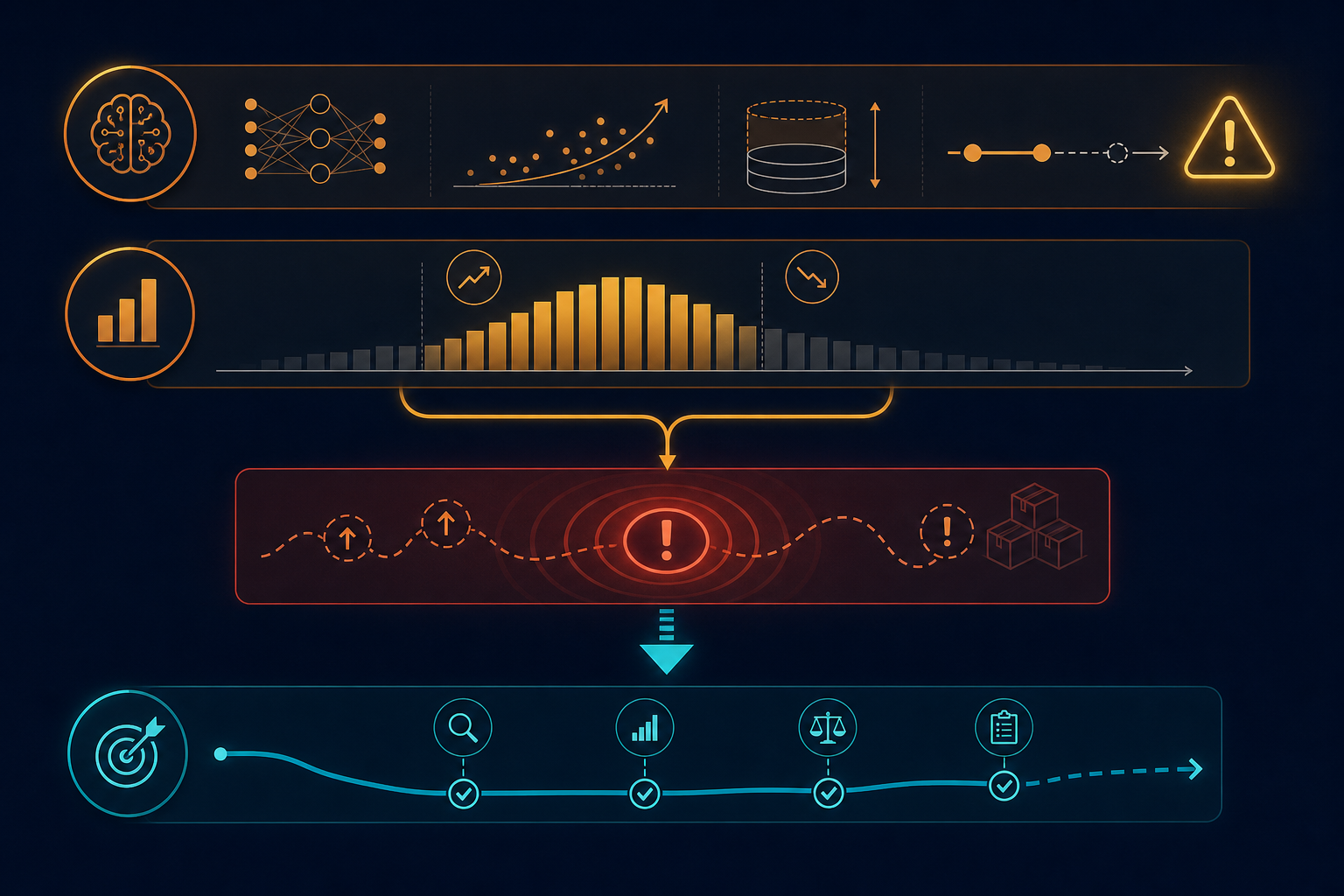
The operational change for China-linked supply chains is meaningful: landed cost visibility improves, supplier reliability increases with fewer regulatory disruptions, and critical material access is partially restored, reducing the cost premium of alternatives. But the AI planning systems running at most enterprises were not built for this environment. They were built for the one that preceded it.
How AI Planning Systems Encode Lead Time Assumptions
To understand why the Phase 2 deal creates a recalibration problem, you need to understand how AI planning systems actually store and use lead time assumptions — because the answer is less dynamic than most vendor marketing suggests.
There are two fundamentally different architectures in deployed systems. The first uses static default parameters: manually configured values for China transit days, safety stock multipliers, supplier lead time buffers, and alternative sourcing cost penalties. These values are set during implementation, updated during periodic planning cycles, and otherwise remain fixed until a planner or system administrator changes them. The second uses ML-updated dynamic parameters: machine learning models that continuously update lead time estimates as new supplier performance data arrives, self-correcting when the model's predictions diverge from actual outcomes.
The gap between these two approaches is the core of the stale assumption problem. As GAINSystems describes, traditional lead time models treat lead time as a static value based on historical averages — an assumption that requires a degree of stability that no longer exists in volatile trade environments. ML-based systems, by contrast, are self-correcting: if a model consistently underestimates lead times for a particular supplier during peak season, subsequent data signals the error and the model adjusts. But this self-correction only works if the incoming data reflects current conditions — not the disrupted conditions that shaped the training data.
The deployment reality matters here. Even platforms marketed as dynamically adaptive — Kinaxis, Blue Yonder, o9 Solutions, SAP IBP — are typically deployed with substantial static parameter layers. Tariff rates, sourcing origin weights, and total landed cost inputs are not fields that AI models update autonomously; they require human input or structured data feeds. When trade conditions change sharply, as they did in both directions during 2025, these parameters become stale unless someone explicitly updates them.
- Static parameters: China transit days, safety stock multipliers, alternative sourcing cost penalties, supplier lead time buffers — typically set during implementation, updated by planners during review cycles.
- Semi-static parameters: Supplier risk scores, country-of-origin weighting, tariff rate inputs — updated when planners or procurement teams trigger a review, not continuously.
- Dynamic ML-updated parameters: Demand signals, short-term forecast adjustments, anomaly detection outputs — self-correcting on new transactional data, but only as good as the underlying data quality and recency.
If your organization is still evaluating whether to deploy an AI planning system, the AI demand planning implementation readiness checklist covers pre-deployment organizational prerequisites. This article addresses a different problem: what happens to the assumptions inside AI systems already running in production when the conditions they were configured for no longer exist.
The Assumption Set That Went Stale After the Phase 2 Deal
During peak 2025 tariff disruption, supply chain planning teams made rational decisions: they extended China lead time buffers, built elevated safety stock, penalized China sourcing in total cost models, and in some cases explicitly de-prioritized Chinese suppliers in replenishment logic. These decisions were encoded into AI planning systems — either as manually updated parameters or as model training data reflecting the disrupted operating environment.
The McKinsey supply chain risk survey (December 2025, n=100 global supply chain companies) documents the scale of this encoding: 45% of companies facing tariff impacts increased inventories as a mitigation measure, 39% pursued dual sourcing strategies, and 33% developed supplier nearshoring or onshoring plans. These are not abstract policy positions — they are operational postures that translated directly into AI planning system parameters and baseline inventory levels.
With the Phase 2 framework in place, several of those parameter sets are now misaligned with current China sourcing economics. Here is the specific assumption set that warrants audit:
| Parameter | What Was Encoded During Peak Disruption | Current Condition Post-Phase 2 | Staleness Risk |
|---|---|---|---|
| China supplier lead time (days) | Extended transit buffers reflecting port congestion, customs delays, and routing uncertainty | Transit times compressing as disruption eases; cargo arriving earlier than planned (Xeneta, 2026) | High — over-buffered lead times generate premature replenishment orders |
| Safety stock multipliers | Elevated buffers sized for ~57% effective tariff rate volatility and supply uncertainty | Effective rate now ~47%; landed cost economics improved | High — excess safety stock ties up working capital unnecessarily |
| Alternative sourcing cost penalties | Near-shoring and dual-sourcing premiums encoded as default routing preferences | China cost advantage partially restored; premium may now overstate actual differential | Medium-High — AI continues routing to higher-cost alternatives |
| China supplier risk / priority scores | Lowered priority scores or explicit de-prioritization in replenishment logic | Supplier performance and cost competitiveness have improved under stabilized conditions | Medium — missed re-engagement windows as AI routes around viable suppliers |
| Total landed cost model inputs | Tariff rate inputs set at ~57% effective rate | MoFo estimates current effective rate at ~47%; fentanyl tariff reduced 10 points | High — every landed cost comparison overstates China cost disadvantage |
| Critical mineral sourcing alternatives | High-cost alternative suppliers weighted heavily due to China export control risk | General licenses issued for gallium, germanium, graphite, rare earths (with caveats) | Medium — alternative sourcing premiums may no longer be justified at prior weighting |
The New Horizon AI dual-track inventory strategy — minimize China safety stock to avoid high-cost inventory, stockpile non-China goods within tariff windows — illustrates the planning logic that drove these encodings during 2025. That logic was rational under ~57% effective tariff conditions. Under ~47% conditions with a 12-month stability horizon, it produces systematically distorted replenishment signals.
The Q2 2026 Compounding Distortion
Stale AI model parameters alone would be a manageable problem. What makes Q2 2026 particularly dangerous is that a second distortion compounds the first — and both errors point in the same wrong direction simultaneously.

The second distortion is the Q1 2026 front-loading hangover. US ports — particularly Los Angeles and Long Beach — absorbed record inbound container volumes in Q1 2026 as importers pre-bought three to six months of supply at the then-prevailing tariff rates. This was rational individual behavior. Its collective consequence is that Q2 2026 year-over-year demand comparisons are now made against an artificially inflated Q1 baseline.
When AI demand models compare Q2 2026 orders against Q1 2026 actuals, they see apparent demand weakness — even where underlying consumption is stable or growing. The front-loaded inventory is sitting in warehouses and distribution centers, suppressing near-term replenishment orders. The AI model interprets this as a demand signal, not as an inventory positioning artifact.
Xeneta adds a logistics timing dimension that compounds this further: supply chains that recalibrated around longer China lead times may face temporary imbalances when transit times compress. Cargo arriving earlier than the AI model expects puts pressure on warehouse capacity, inland transport, and inventory planning — even when the underlying economics are improving.
What Happens When Planners Act on Stale AI Recommendations
The business risk is concrete. Three failure modes are most likely for planning teams running unrecalibrated AI systems through Q2 and Q3 2026.
- Inventory overcapitalization. Safety stock buffers sized for ~57% tariff economics continue generating replenishment orders that are no longer justified by landed cost volatility. The AI model continues recommending elevated buffer levels because its safety stock multipliers were set during peak disruption and have not been updated. Capital is tied up in inventory that exists to hedge a risk that has partially resolved.
- Missed China cost re-engagement windows. AI models that de-prioritized China suppliers during peak 2025 disruption continue routing replenishment to higher-cost near-shored or dual-sourced alternatives. The total landed cost model still shows China at ~57% effective tariff rates. Procurement teams acting on these recommendations forgo the improved cost position that the Phase 2 framework created — while competitors who recalibrated earlier capture the margin advantage.
- Misaligned replenishment signals from front-load distortion. AI demand models reading Q2 2026 orders against the inflated Q1 baseline project demand weakness and recommend inventory drawdown. If planners execute these recommendations — marking down excess inventory, reducing forward orders — they risk stockouts in Q3 and Q4 when the front-loaded inventory is consumed and underlying demand reasserts itself.
The Kinaxis data point is instructive here. Kinaxis reported a 124% increase in scenario usage among its customers following the April 2025 tariff shock — evidence that planning teams invested heavily in disruption-direction modeling. But the de-escalation direction has received almost no equivalent investment. The scenario infrastructure exists; the recalibration work has not been done.
SPS Commerce documents the safety stock dimension directly: buffers built on tariff-era assumptions can be miscalibrated once landed cost improves. The instinct to hold more inventory ahead of cost increases made sense in 2025. Running that same logic into a stabilized tariff environment produces unnecessary working capital drag.
How Leading Teams Are Recalibrating: Manual Updates vs. Dynamic Tools
Planning teams have two recalibration paths available, and the right choice depends primarily on what their deployed system actually supports — not what the vendor markets.
Manual Parameter Update Cycle
For most deployed enterprise AI planning systems, recalibration means a structured manual update process: identify which parameters were set during peak disruption conditions, source current data (actual China transit times, current landed cost calculations at ~47% effective rate, current supplier performance), update static values in the planning system, and re-run affected scenarios. This is not a one-time event — it requires a disciplined review cycle, particularly while the Phase 2 framework is in its first six months.
Dynamic AI Recalibration
ML-based lead time sensing, as described by GAINSystems, offers a self-correcting alternative: as new supplier performance data arrives, the model updates its lead time estimates without requiring manual intervention. But this capability has a prerequisite that most organizations cannot currently meet.
The RAND Corporation found that over 80% of AI projects fail — twice the rate of other IT projects — and the reason is rarely the model; it is almost always the data underneath.
The Forbes/RAND finding points to the actual bottleneck for most organizations attempting recalibration: master data quality, not model capability. Supplier records in most enterprise systems were built to answer two questions — who do we pay, and where do we send the PO. They were not built to track country-of-processing distinctions for tariff classification, or to distinguish between supplier locations at the granularity that 2025-era export controls required. Before dynamic AI recalibration can work, the underlying supplier coding, tariff classification, and origin attribution data must be accurate and current.
For CPG and retail operators, the recalibration challenge is further compounded by promotional calendars and retailer OTIF commitments built on pre-deal cost structures. The AI demand forecasting CPG and retail use case provides sector-specific context on how these constraints interact with forecast model assumptions.
Which AI Planning Platforms Handle Assumption Drift Better
Platform architecture matters for recalibration speed, but the gap between marketed capability and deployment reality is significant. Here is an honest assessment of how the major platforms differ on this dimension, based on vendor-reported data and publicly available information.

| Platform | Recalibration Architecture | Deployment Reality | Relevant Capability Note |
|---|---|---|---|
| Kinaxis | Concurrent planning with scenario modeling; parameter changes can propagate across planning models | Customers increased scenario usage 2x in Q2 2025 and 124% post-April shock — but recalibration direction (de-escalation) has received minimal structured attention (vendor-reported) | Strong scenario architecture for disruption modeling; de-escalation recalibration requires deliberate scenario design, not automatic |
| Blue Yonder | Integrated demand and supply planning; parameter updates flow through connected plan layers | Enterprise deployments typically require manual parameter update cycles for tariff rate inputs and lead time buffers | See the Blue Yonder vs. Kinaxis comparison for architecture differences on scenario modeling |
| o9 Solutions | Connected data graph architecture positions cross-model assumption updates as a design advantage | Data graph connectivity depends on data quality of underlying supplier and cost records — the same master data constraint applies | Connected graph can accelerate parameter propagation once source data is corrected; does not resolve classification debt automatically |
| SAP IBP | Integrated with S/4HANA master data; parameter updates inherit ERP data quality | Tariff rate inputs and origin-based cost calculations require structured master data updates; IBP does not auto-update from trade policy changes | Tight ERP integration is an advantage for organizations with clean master data; a liability for those with legacy classification issues |
The Recalibration Checklist: Parameters to Audit, Sequence, and Thresholds
The following framework is structured as a sequenced audit. Work through it in order — parameters earlier in the sequence affect the validity of parameters later in the sequence. Do not start with safety stock multipliers before you have corrected the total landed cost inputs those multipliers depend on.
Step 1: Total Landed Cost Model — Tariff Rate Inputs
This is the foundational parameter. Every downstream calculation — safety stock sizing, alternative sourcing cost comparison, China supplier scoring — depends on the landed cost differential between China-origin and alternative-origin goods. If this input is wrong, everything downstream is wrong.
- Update the effective tariff rate input from ~57% to ~47% (MoFo estimate for post-Phase 2 average). Note: this is an average across product categories — Section 301 rates vary by HTS code. Update at the SKU or category level where possible.
- Distinguish between the Geneva reciprocal rate (reduced from 30% to 20% after fentanyl tariff reduction) and total effective rate (which includes pre-existing Section 301 levies). The ~47% figure is the total effective rate, not the reciprocal rate alone.
- Verify Section 301 exclusion status for any SKUs where exclusions were extended through November 10, 2026. These items may have a lower effective rate than the category average.
- Flag critical mineral inputs (gallium, germanium, graphite, rare earths) for separate review given the MoFo ambiguity on partial export control persistence.
Step 2: China Supplier Lead Time Parameters
Compare the lead time values currently encoded in your planning system against actual supplier performance data from the past 60–90 days. The question is not what lead times were during peak disruption — it is what they are now.
- Pull actual transit times from your TMS or freight visibility platform for China-origin shipments over the past 60 days. Compare against the encoded lead time values in your planning system.
- If encoded lead times exceed actual performance by more than your standard variability buffer, update the base value. Do not eliminate the variability buffer — transit time compression can create warehouse timing problems even when average lead times improve.
- For suppliers where you have no recent shipment data (because they were de-prioritized during 2025), use carrier-reported transit time data for the relevant lanes as a proxy until supplier performance data accumulates.
Step 3: Safety Stock Multipliers
Recalculate safety stock levels using the updated landed cost inputs from Step 1 and the updated lead time variability from Step 2. The question is whether the current multipliers reflect current volatility — not peak 2025 volatility.
- Identify SKUs where safety stock was increased specifically as a tariff hedge (not as a demand variability buffer). These are the first candidates for reduction.
- Recalculate safety stock using current lead time variability and current service level targets. Do not use peak-disruption variability figures if actual variability has declined.
- Apply reductions gradually — staged drawdown over 4–6 weeks — rather than immediate bulk reduction, to avoid creating replenishment gaps if actual demand is stronger than the front-load-distorted baseline suggests.
Step 4: Alternative Sourcing Cost Penalties and Routing Weights
Verify whether the cost premiums encoded for near-shored and dual-sourced alternatives still reflect actual cost differentials at current China landed costs. Many of these premiums were calculated against ~57% effective tariff rates.
- Recalculate the cost differential between China-origin and alternative-origin for your top 20 SKUs by spend. Use current freight rates, current tariff inputs, and current supplier quotes.
- Update routing weights in the AI planning model to reflect revised differentials. Where China has regained cost competitiveness, the model should be able to route replenishment there — if it currently cannot, the routing constraint is a parameter, not a market reality.
- Do not eliminate near-shoring or dual-sourcing infrastructure. The Phase 2 framework is a 12-month window, not a permanent resolution. Maintain the sourcing optionality; adjust the cost weights.
Step 5: Demand Baseline Normalization for Q1 Front-Loading
This step addresses the second distortion. Identify SKUs where Q1 2026 order volumes were materially elevated by tariff front-loading, and apply correction factors before running Q2 and Q3 forecasts against those baselines.
- Identify front-loaded SKUs: look for items with China origin, Q1 2026 order volumes significantly above trend, and current inventory levels above typical coverage targets. These are the SKUs where the baseline distortion is most acute.
- For affected SKUs, use a normalized baseline that excludes the front-load spike — typically the 12-month trailing average excluding Q1 2026, or a seasonally adjusted trend line. Do not let the AI model use Q1 2026 actuals as the comparison period for Q2 and Q3 forecasts without adjustment.
- Flag these SKUs in your planning system so that AI-generated replenishment recommendations for them receive human review before execution through at least Q3 2026.
Step 6: Maintain the Re-Escalation Scenario Set
Recalibration to Phase 2 conditions should not mean discarding the disruption-era parameter set. Given the scenario probabilities — 10% full snap-back to 100%+ tariffs, 20% partial re-escalation to 60–80% — planning teams need to be able to switch back to disruption-era assumptions quickly if conditions change.
- Save the current disruption-era parameter set as a named scenario in your planning system before overwriting any values. Label it with the date and the conditions it was calibrated for.
- Define the trigger conditions that would prompt a switch back to the disruption scenario: specific tariff announcements, Section 301 exclusion non-renewal, critical mineral export control reimposition.
- Run both scenarios — Phase 2 stable and re-escalation — in parallel on a monthly basis through at least Q3 2026. The gap between the two scenario outputs is your policy uncertainty exposure.
The planning teams that will capture the most value from the Phase 2 window are not those that move fastest to recalibrate — they are those that recalibrate most accurately, with the clearest view of which parameters are stale, which are still valid, and which need to be maintained in parallel for the scenario that has not yet resolved.
Comments
Join the discussion with an anonymous comment.